User Guide#

An investment plan covers a time period. It has an associated portfolio. A portfolio includes a set of assets and their associated weights.

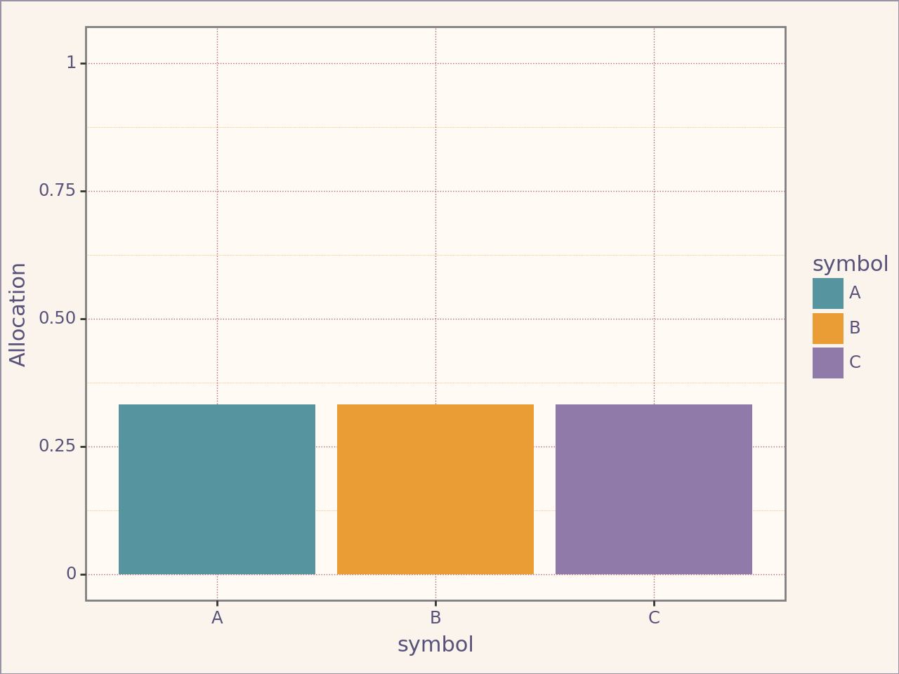
Let’s define our plan. We are interested in knowing what we would have earned if we invested equal weights in companies A, B and C. Starting on January up to today (2025-05-02).

Defining a Portfolio#

from portfolio_plan import Assets, Weights, Asset, Portfolio, Frequency
from portfolio_plan.resource import File
from portfolio_plan.data import example_prices_path


portfolio = Portfolio(
    assets=Assets(
        [Asset("A"), Asset("B"), Asset("C")],
        resource=File(path=example_prices_path(), frequency=Frequency.BDAILY),
    ),
    name="Portfolio",
    weights=Weights(),  # No parameter means equal weights across assets
)

portfolio.plot_allocation()

../_images/cc1fd135247b51866f707989d7cb05314dcc0ada232441e5518d5b203a2e31ec.png

<Figure Size: (640 x 480)>

Defining a Plan#

from portfolio_plan import Plan
from datetime import datetime


plan1 = Plan(
    portfolio=portfolio,
    start_date=datetime.strptime("2025-01-30", "%Y-%m-%d"),
    end_date=datetime.strptime("2025-03-01", "%Y-%m-%d"),
)
plan1

------------------------------------------------------------
| Plan for period 2025-01-30 00:00:00, 2025-03-01 00:00:00 |
------------------------------------------------------------
| A                                                        |
------------------------------------------------------------
| B                                                        |
------------------------------------------------------------
| C                                                        |
------------------------------------------------------------

Returns#

Individual Returns#

returns = plan1.returns(portfolio.name) # Returns object
returns

-----------------------------------------------------------------
| Returns for period 2025-01-30 00:00:00 to 2025-02-28 00:00:00 |
-----------------------------------------------------------------
| A                                                             |
-----------------------------------------------------------------
| B                                                             |
-----------------------------------------------------------------
| C                                                             |
-----------------------------------------------------------------

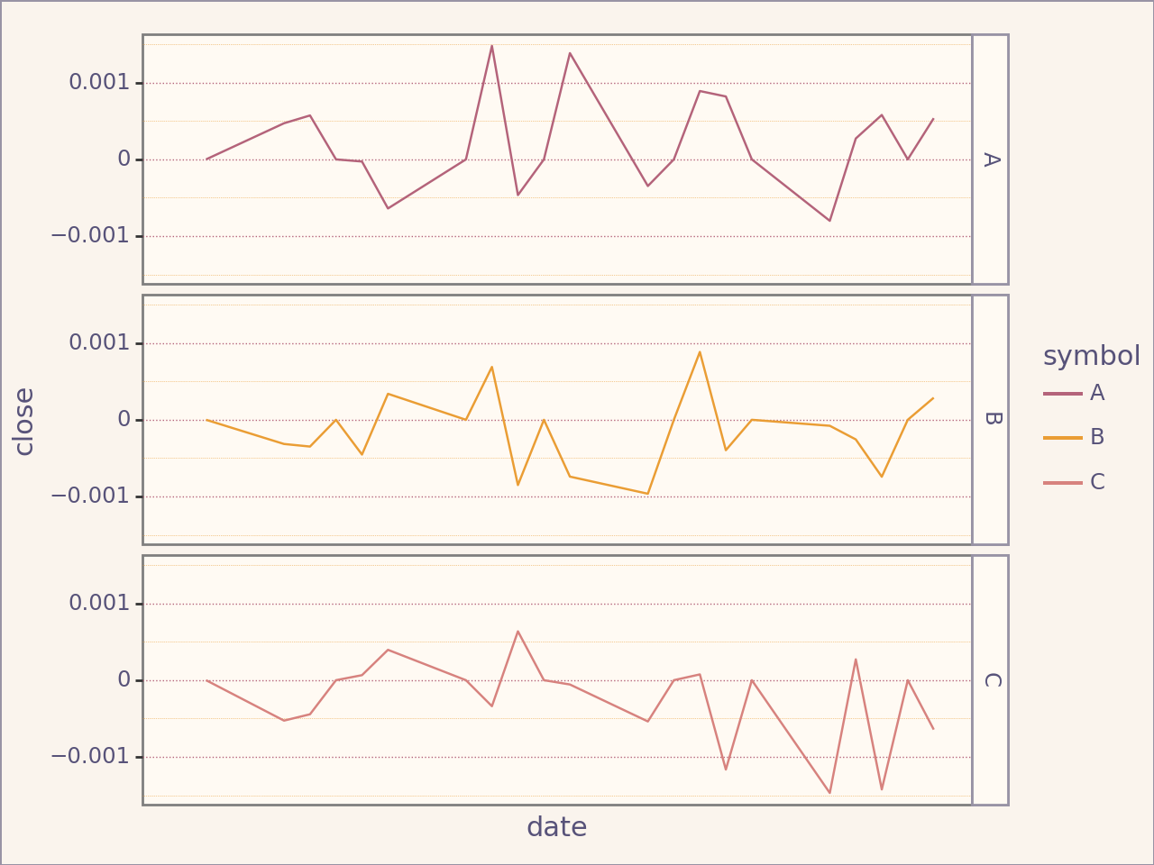
If we wish to plot the returns:

returns.plot_close()

/home/runner/work/portfolio-plan/portfolio-plan/.venv/lib/python3.10/site-packages/plotnine/geoms/geom_path.py:98: PlotnineWarning: geom_path: Removed 1 rows containing missing values.

../_images/7fe9377bf6d12ff06f4e2c543bd21124a6734a369a310f66863fbb08efca7a85.png

<Figure Size: (640 x 480)>

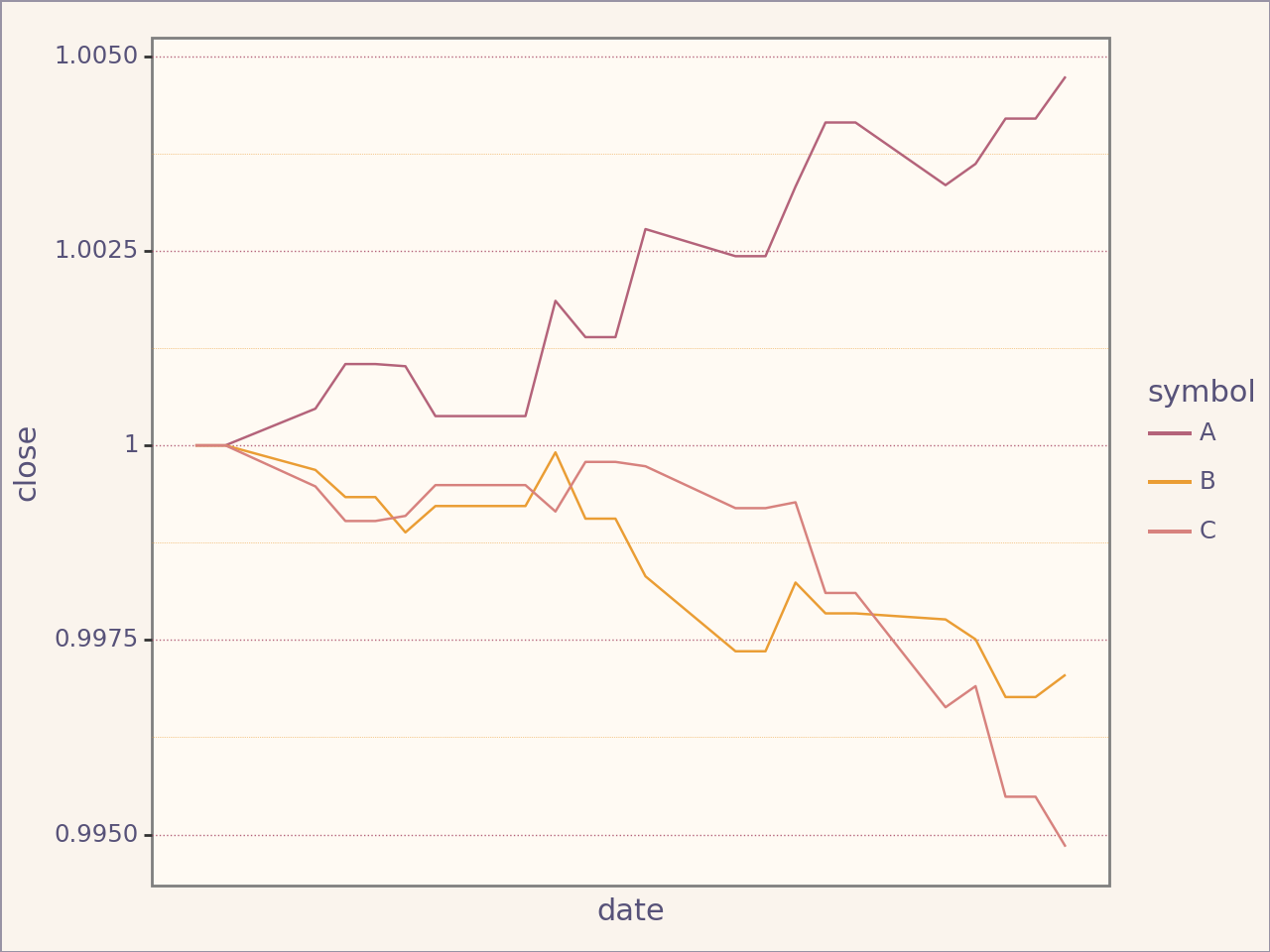
Or the cumulative returns:

cumulative_returns = returns.cumulative("Cumulative")
cumulative_returns.plot_close()

../_images/1db47c620096e92ba1e31f8496650dbee66f83edc93fd71e5e8eece5b42584ee.png

<Figure Size: (640 x 480)>

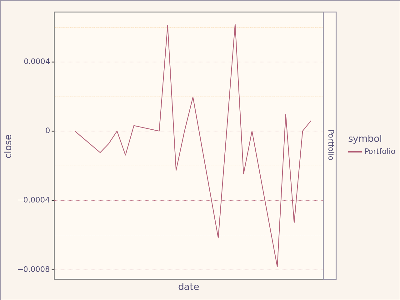
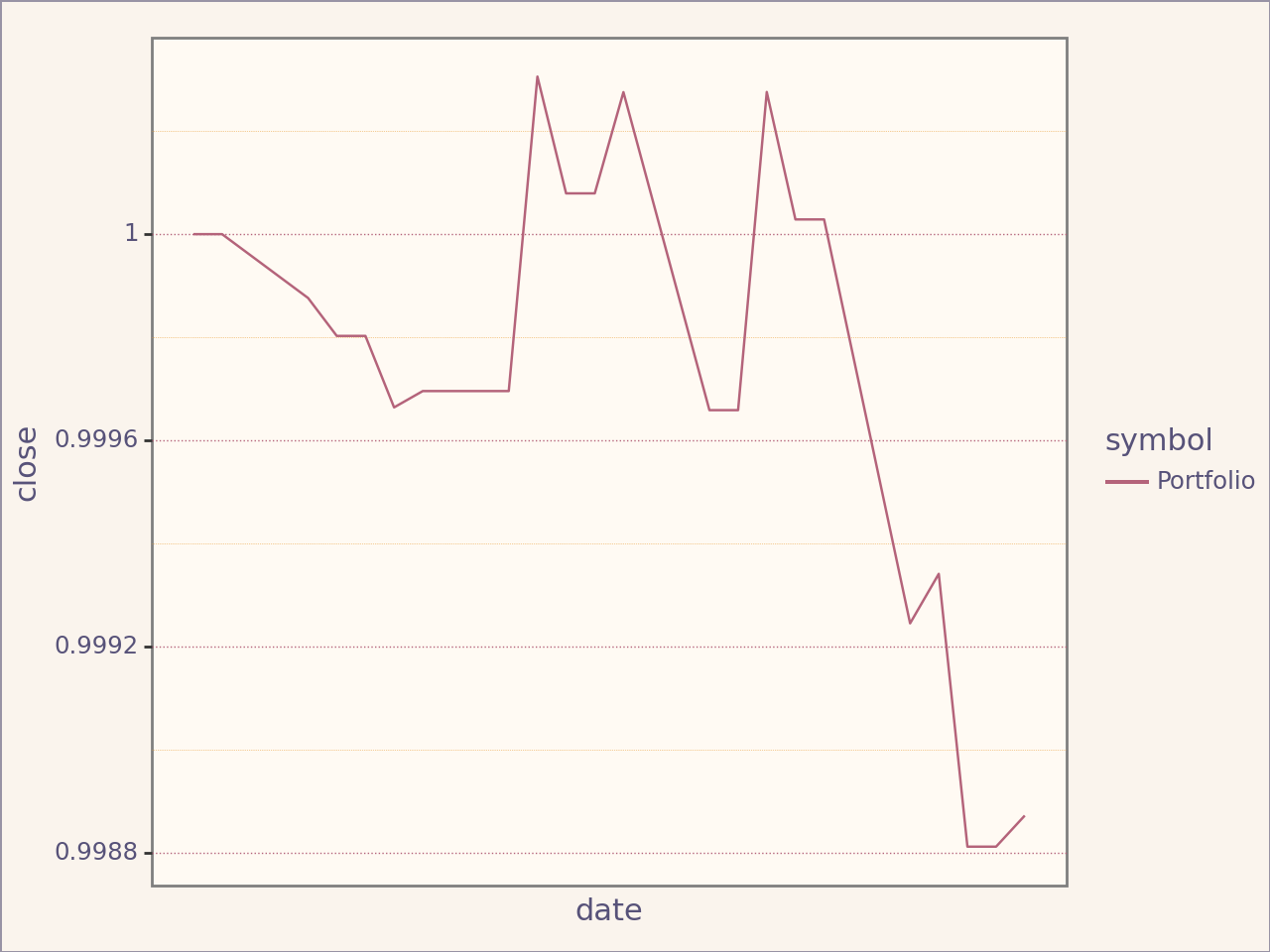
Portfolio Returns#

portfolio_returns1 = plan1.portfolio_returns()
portfolio_returns1.plot_close()

/home/runner/work/portfolio-plan/portfolio-plan/.venv/lib/python3.10/site-packages/plotnine/geoms/geom_path.py:98: PlotnineWarning: geom_path: Removed 1 rows containing missing values.

../_images/c339dd1cf56a992350dc3890faf17749dcc0bf9b1c50e07cf5c37872632e1aea.png

<Figure Size: (640 x 480)>

Cumulative Portfolio Returns:

cumulative_portfolio_returns1 = portfolio_returns1.cumulative("Cumulative")
cumulative_portfolio_returns1.plot_close()

../_images/86a92e93a18b80de0167d606839da866a16fe7c0902f9c1341fddcbe26b388ee.png

<Figure Size: (640 x 480)>

Combining plans#

You might be interested in the joined returns of two investment plan happening at different timeframe.

plan2 = Plan(
    portfolio = portfolio,
    start_date = datetime.strptime("2025-03-02", "%Y-%m-%d"),
    end_date = datetime.strptime("2025-05-05", "%Y-%m-%d")
)
print(plan1)
print(plan2)

------------------------------------------------------------
| Plan for period 2025-01-30 00:00:00, 2025-03-01 00:00:00 |
------------------------------------------------------------
| A                                                        |
------------------------------------------------------------
| B                                                        |
------------------------------------------------------------
| C                                                        |
------------------------------------------------------------
------------------------------------------------------------
| Plan for period 2025-03-02 00:00:00, 2025-05-05 00:00:00 |
------------------------------------------------------------
| A                                                        |
------------------------------------------------------------
| B                                                        |
------------------------------------------------------------
| C                                                        |
------------------------------------------------------------

portfolio_returns2 = plan2.portfolio_returns()

cumulative_portfolio_returns2 = portfolio_returns2.cumulative("Cumulative")

The >> operator enables easy creation of joined plan.

joinedplan = plan1 >> plan2
joinedplan

                                                           ┌────────────┐
                                                           │ JoinedPlan │
                                                           └──────┬─────┘
                                                                  │
                                ┌─────────────────────────────────┴─────────────────────────────────┐
┌───────────────────────────────┴──────────────────────────────┐    ┌───────────────────────────────┴──────────────────────────────┐
│ ------------------------------------------------------------ │    │ ------------------------------------------------------------ │
│ | Plan for period 2025-01-30 00:00:00, 2025-03-01 00:00:00 | │    │ | Plan for period 2025-03-02 00:00:00, 2025-05-05 00:00:00 | │
│ ------------------------------------------------------------ │    │ ------------------------------------------------------------ │

joinedplan.plot_allocations()

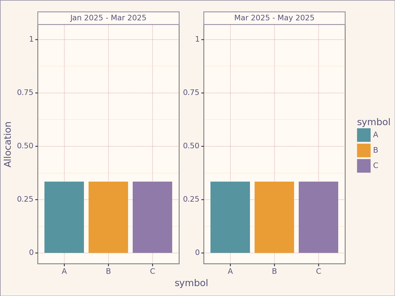
../_images/dd9d289726d6f7d8bb9e8b38f83ef5747c2b1c104cb48afc71f004fa7670a59c.png

<Figure Size: (640 x 480)>

Note: Plans have to be placed by order of timeframe, otherwise an error will be raised.

from portfolio_plan.errors import PeriodOverlapError


try:
    plan2 >> plan1
except PeriodOverlapError as e:
    print(e)

Plans can not overlap in time period and must be ordered by time period

Interested in what is the return on investment of a joined plan ?

joinedplan_cumulative_returns = joinedplan.portfolio_cumulative_returns("Joined Plan")
joinedplan_cumulative_returns.data

	CumulativeReturns	open	close	high	low
symbol	date
Portfolio	2025-01-30	1.000000	1.000000	1.000000	1.000000
	2025-01-31	1.000000	1.000000	1.000000	1.000000
	2025-02-03	0.999746	0.999876	0.999939	0.999918
	2025-02-04	0.999591	0.999803	0.999903	0.999870
	2025-02-05	0.999591	0.999803	0.999903	0.999870
	...	...	...	...	...
	2025-04-29	1.001401	1.000794	1.000421	1.000551
	2025-04-30	1.001095	1.000649	1.000350	1.000456
	2025-05-01	1.000904	1.000531	1.000286	1.000372
	2025-05-02	1.000904	1.000531	1.000286	1.000372
	2025-05-05	1.000310	1.000239	1.000141	1.000179

68 rows × 4 columns

joinedplan_cumulative_returns.data.loc["Portfolio"].head()

CumulativeReturns	open	close	high	low
date
2025-01-30	1.000000	1.000000	1.000000	1.000000
2025-01-31	1.000000	1.000000	1.000000	1.000000
2025-02-03	0.999746	0.999876	0.999939	0.999918
2025-02-04	0.999591	0.999803	0.999903	0.999870
2025-02-05	0.999591	0.999803	0.999903	0.999870

from plotnine import scale_x_datetime


(
    joinedplan_cumulative_returns.plot_close(scale_x=False) + # Define scale manually
    scale_x_datetime(date_breaks="1 week", date_labels="%Y-%m-%d")
)

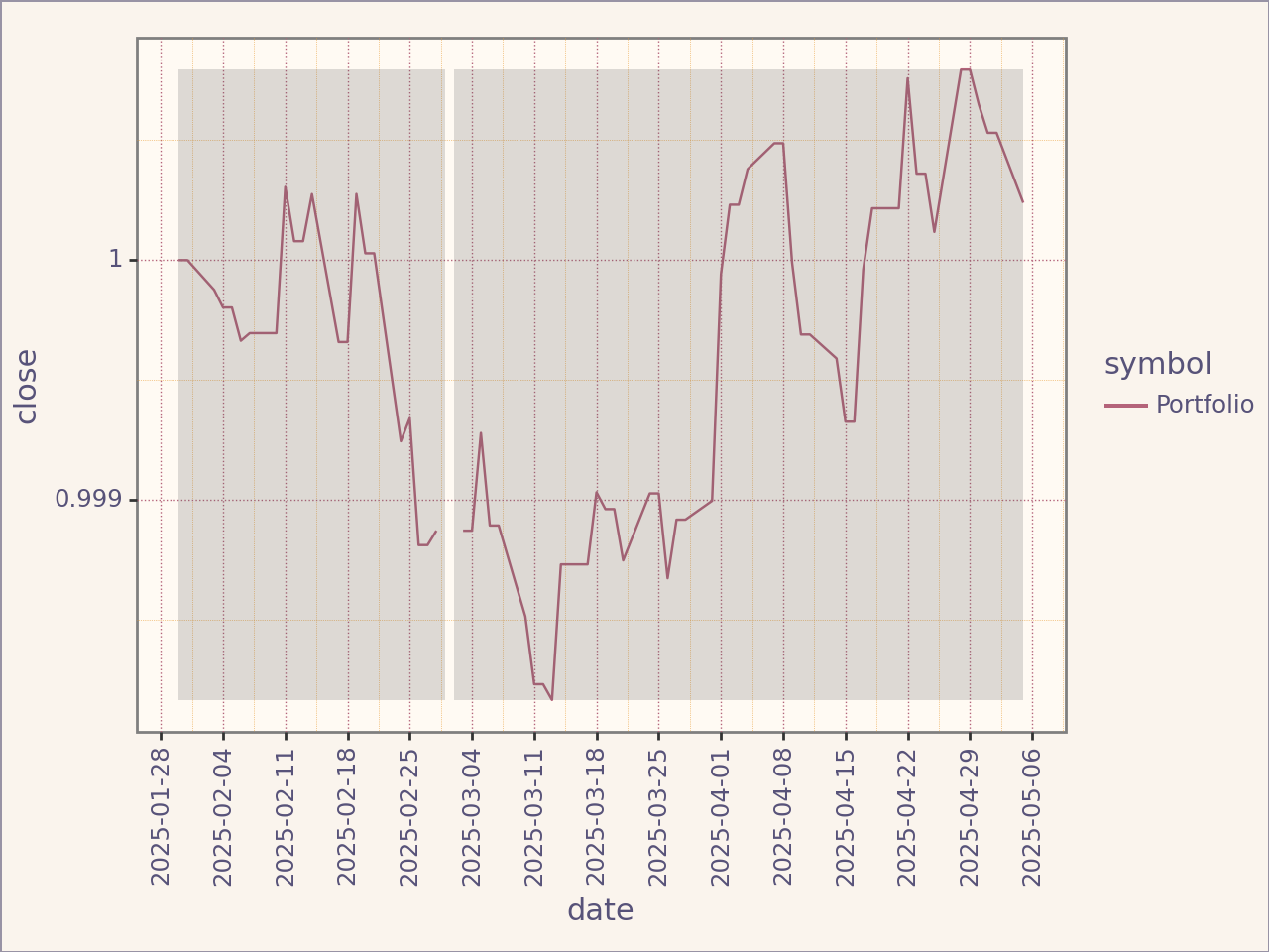
../_images/19730ca4143ce7ab3e08ef820eeaaeed9b796952098adb3d425a86dea794a086.png

<Figure Size: (640 x 480)>

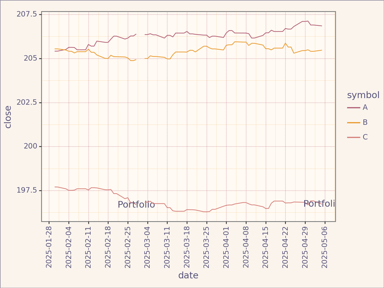
Comparing FinancialSeries#

You might want to compare each returns, prices

Prices#

from portfolio_plan.financialseries import Comparison


comparison = Comparison(
    [plan1.prices(), plan2.prices()]
)
(
    comparison.plot_close(scale_x=False)
    + scale_x_datetime(date_breaks="1 week", date_labels="%Y-%m-%d")
)

/home/runner/work/portfolio-plan/portfolio-plan/.venv/lib/python3.10/site-packages/plotnine/layer.py:364: PlotnineWarning: geom_text : Removed 65 rows containing missing values.
/home/runner/work/portfolio-plan/portfolio-plan/.venv/lib/python3.10/site-packages/plotnine/layer.py:364: PlotnineWarning: geom_text : Removed 137 rows containing missing values.

../_images/3b7ce2756b3c8f0dd0be803e0381e3cba9a8fb59340c6ba3f002725d1e408d5d.png

<Figure Size: (640 x 480)>

Returns#

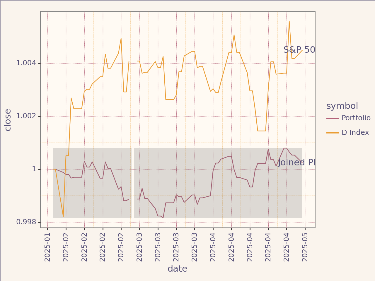
Instead of comparing prices, you want to compare returns. You may want to look at how your strategy differs with an index fund for example

Non-Cumulative#

# NOT YET IMPLEMENTED

Cumulative#

We start by defining the benchmark plan (note that this is only necessary for multiple period investments).

from portfolio_plan.financialseries import Comparison


assets = Assets(
    [Asset("^D")],
    resource=File(path=example_prices_path(), frequency=Frequency.BDAILY),
)

benchmark = Portfolio(
    assets=assets,
    weights=Weights(),
    name="D Index"
)
benchmark_plan_1 = Plan(
    portfolio=benchmark,
    start_date=datetime.strptime("2025-01-30", "%Y-%m-%d"),
    end_date=datetime.strptime("2025-03-01", "%Y-%m-%d"),
)

benchmark_plan_2 = Plan(
    portfolio = benchmark,
    start_date = datetime.strptime("2025-03-02", "%Y-%m-%d"),
    end_date = datetime.strptime("2025-05-05", "%Y-%m-%d")
)

benchmark_joined = benchmark_plan_1 >> benchmark_plan_2

comparison = Comparison(
    [
        joinedplan.portfolio_cumulative_returns("Joined Plan"),
        benchmark_joined.portfolio_cumulative_returns("S&P 500")
    ]
)

(
    comparison.plot_close(scale_x=False) +
    scale_x_datetime(date_breaks="1 week", date_labels="%Y-%m")
)

/home/runner/work/portfolio-plan/portfolio-plan/.venv/lib/python3.10/site-packages/plotnine/layer.py:364: PlotnineWarning: geom_text : Removed 67 rows containing missing values.
/home/runner/work/portfolio-plan/portfolio-plan/.venv/lib/python3.10/site-packages/plotnine/layer.py:364: PlotnineWarning: geom_text : Removed 67 rows containing missing values.

../_images/db84f7b3ff5170b6bf5797a751d34fe37b67f5937066ad4342d6be423408fc0d.png

<Figure Size: (640 x 480)>

Information Ratio#

It is possible to calculate the information ratio between two plan. Since each ratio corresponds to a specific investment plan, no annualization is performed. Plans must have the same starting period or ending period.

from portfolio_plan.ratios import InformationRatio


ir = InformationRatio(plan1, benchmark_plan_1)
ir_returns1 = ir.period_returns()  # Returns a singleton dataframe
assert ir_returns1.is_singleton
ir_returns1

-----------------------------------------------------------------
| Returns for period 2025-02-28 00:00:00 to 2025-02-28 00:00:00 |
-----------------------------------------------------------------
| IR: Portfolio-D Index                                         |
-----------------------------------------------------------------

ir = InformationRatio(plan2, benchmark_plan_2)
ir_returns2 = ir.period_returns()
assert ir_returns2.is_singleton
ir_returns2

-----------------------------------------------------------------
| Returns for period 2025-05-05 00:00:00 to 2025-05-05 00:00:00 |
-----------------------------------------------------------------
| IR: Portfolio-D Index                                         |
-----------------------------------------------------------------

ir_returns1.data

		open	low	high	close
symbol	date
IR: Portfolio-D Index	2025-02-28	-0.256186	-0.252886	-0.252465	-0.253722

ir_returns1.data

		open	low	high	close
symbol	date
IR: Portfolio-D Index	2025-02-28	-0.256186	-0.252886	-0.252465	-0.253722

Information Ratio Returns are always singletons.

User Guide#

Defining a Portfolio#

Defining a Plan#

Returns#

Individual Returns#

Portfolio Returns#

Combining plans#

Comparing FinancialSeries#

Prices#

Returns#

Non-Cumulative#

Cumulative#

Information Ratio#

This Page